Light Field Imaging
This page introduces the physical foundations of light field imaging. It is independent of a particular camera; How LumiScan X Works describes how the LumiScan X applies these principles. The publications cited are listed in References.
What Is Light Field Imaging?
Light field imaging is a computational imaging technique that records not only the intensity of the light arriving at an image sensor, but also the directions from which it arrives. A conventional camera integrates the light from all directions in each pixel and records a two-dimensional projection of the three-dimensional scene; most of the directional information is lost. A light field camera preserves part of it by observing the scene from several viewpoints: it samples the light rays by both their position and their direction.
This additional information enables:
-
Depth estimation: determining the distance between the camera and the visible surfaces.
-
3D reconstruction: recovering the three-dimensional geometry of objects.
-
Digital refocusing: changing the focal plane computationally after the image has been taken.
-
Perspective synthesis: generating views from viewpoints within or near the captured angular range.
-
Occlusion handling: recovering surfaces that are hidden from some viewpoints but visible from others.
This makes light field imaging attractive for industrial tasks that need reliable three-dimensional information.
The Plenoptic Function
The theoretical basis of light field imaging is the plenoptic function (Adelson and Bergen, 1991). It describes the light present at every position in space, in every direction, at every wavelength and at every point in time:
| Parameter | Description |
|---|---|
\(x, y, z\) |
Position in three-dimensional space |
\(\theta, \phi\) |
Direction of light propagation |
\(\lambda\) |
Wavelength of the light |
\(t\) |
Time |
The plenoptic function is therefore a seven-dimensional description of the light in a scene. If it were known completely, the view from any position in any direction could be synthesized. Measuring all seven dimensions is not practical, so light field cameras capture a subset of the plenoptic function under specific assumptions.
Reduction to Four Dimensions
For machine vision, the following assumptions usually hold:
-
The scene is observed at one point in time.
-
The measurement uses a defined spectral range.
-
Light propagates along straight rays through a homogeneous medium.
-
Absorption and scattering between the object and the camera are negligible.
Under these conditions, the radiance along a ray in free space is constant, so the position along the ray does not have to be represented. The description reduces to four dimensions: the four-dimensional light field, the mathematical basis of most practical light field cameras.
The Four-Dimensional Light Field
A convenient representation of the light field is the two-plane parameterization (Levoy and Hanrahan, 1996; Gortler et al., 1996): each ray is described by its intersections with two parallel reference planes (Two-plane parameterization: each ray is identified by its intersection points (u, v) and (s, t) with two parallel reference planes.).
Here \((u, v)\) is the intersection of the ray with the first reference plane and \((s, t)\) its intersection with the second. Together, the four coordinates identify an oriented ray.
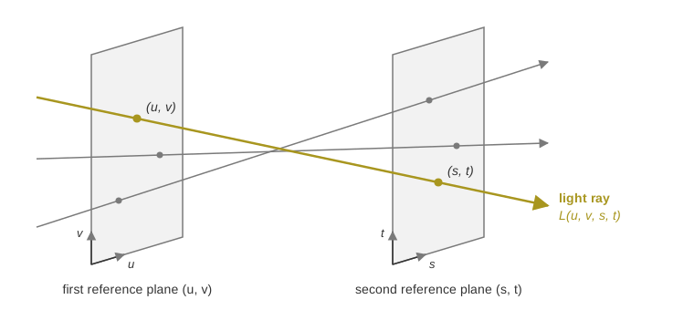
The two planes can be read as viewpoints and image positions, but their exact physical meaning depends on the optical architecture. In a camera array, for example, the first plane can represent the camera positions and the second the position within each camera’s image. Each camera then samples a two-dimensional subset of the four-dimensional light field, and the images of several cameras together provide samples in both the spatial and the angular dimensions.
Spatial and Angular Resolution
Light field imaging has two kinds of resolution:
-
Spatial resolution is the ability to distinguish small features within an image.
-
Angular resolution is the number and distribution of the viewing directions from which the scene is observed.
More angular samples show more of how the appearance of the scene changes with the viewpoint, and this is the information from which depth is reconstructed. Spatial and angular sampling compete for the available measurement resources, and the architectures resolve this differently: microlens-based cameras divide the pixels of one image sensor between spatial and angular sampling, while camera arrays such as the LumiScan X record complete images from several viewpoints on separate image sensors. Light Field Acquisition Architectures compares the two.
From Light Fields to 3D Reconstruction
Depth estimation from a light field relies on parallax: the apparent displacement of an object when it is observed from different viewpoints. Objects close to the camera are displaced more between the viewpoints than distant objects, so measuring the displacement yields the three-dimensional position of the visible scene points.
Parallax, Disparity and Depth
Consider two calibrated cameras with known relative position and orientation that observe the same object point. The point is projected to a different image location in each camera; the displacement between these corresponding image points is the disparity. For a simplified stereo configuration with parallel optical axes, depth and disparity are related by:
| Variable | Description |
|---|---|
\(Z\) |
Distance of the object point from the cameras |
\(f\) |
Focal length of the cameras, in pixels |
\(B\) |
Baseline: the distance between the two camera centers |
\(d\) |
Disparity between the corresponding image points, in pixels |
Depth is therefore inversely proportional to disparity: a point twice as far away shows half the disparity. Light field cameras extend this principle to many viewpoints. They evaluate correspondences across several images instead of two, which adds geometric constraints and can make the depth reconstruction more robust.
Multi-View Reconstruction
A multi-view reconstruction typically involves these steps:
-
Image acquisition: capture images from different viewpoints.
-
Geometric calibration: determine the intrinsic and extrinsic parameters of the cameras.
-
Correspondence: identify the observations that belong to the same scene point.
-
Depth estimation: calculate the depth from the geometry of the corresponding observations.
-
3D reconstruction: generate a depth map or a point cloud.
-
Quality evaluation: identify uncertain or inconsistent measurements.
Depending on the algorithm, correspondence estimation uses local image features, dense matching, cost-volume optimization, epipolar geometry or learned representations. The result is a representation of the scene geometry that subsequent machine vision tasks can use.
Applications
Light field 3D reconstruction supports industrial applications such as:
-
robot guidance and object localization
-
automated bin picking
-
3D inspection and surface reconstruction
-
object recognition and pose estimation
-
dimensional measurement and quality control
The achievable accuracy and robustness depend on the optical configuration, the surface properties, the working distance, the calibration and the reconstruction algorithms.